변수 이름/의미/예시 정리
| no | name | 의미 | 예시 |
| 1 | label | label or class # | label = 16 |
| 2 | height | Input image height(mfcc의 이미지 높이) | height = 48 |
| 3 | width | Input image width(mfcc의 이미지 너비) | width = 173 |
| 4 | SR sample_rate | Hz, 주파수를 의미, 보통 44100 사용 | SR = 44100 |
| 5 | stft | 오디오를 스펙토그램으로 만든 것 | stft = librosa.stft(audio_file) |
| 6 | n_fft | 오디오 프레임 사이즈 | n_fft = 2048 |
| 7 | n_hop hop_length hop_size | window가 움직이는 너비, 프레임 간격 Librosa default is n_fft // 4 ⇒ 512나 256 많이 사용 | hop_length = 512 |
| 8 | mfccs | mfcc 변환 후 feature 벡터 | mfccs = librosa.feature.mfcc(y=audio, sr=sample_rate, n_mfcc=40) |
| 9 | n_mfcc | mfcc만들 때 오디오 신호를 나눌 층 수, 보통 40 | n_mfcc=40 |
| 10 | mfcc.shape | mfcc 계층 수(=n_mfcc), 프레임 수(=오디오/hop_length) | (40, 302) |
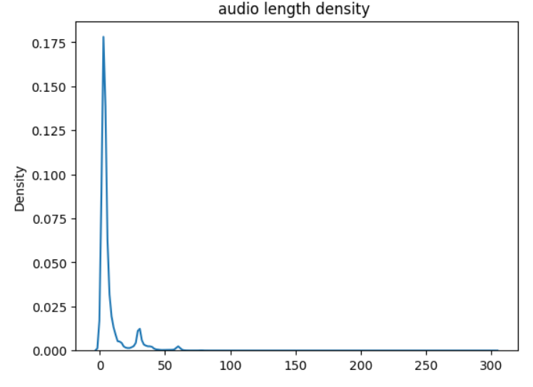
| 11 | len | 음성파일 길이 =오디오 신호 길이/주파수 | librosa.get_duration(y=audio_file, sr=sample_rate) |
| 12 | win_length | frame length |
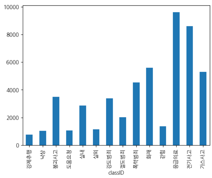
Dataset
: AI hub 위급상황 음성/음향 validation set 약 5만개
Audio -> Feature
def extract_features(file_path): #audio_df[file_path]
    # 예시로 5초를 기준으로 설정하겠습니다.
    reference_length = 5  # 5초

    # 각 파일의 mfccs 특징을 처리하여 동일한 길이로 만듭니다.
    audio, sr = librosa.load(audio_df['file_path'][1], sr=44100, mono=True)
    audio = librosa.util.fix_length(audio, size=5*sr)
    mfccs = librosa.feature.mfcc(y=audio, sr=sr, n_mfcc=40, hop_length=1024, n_fft=2048)
    return mfccs
AIhub model feature
label = 16 # total label
height = 48 # Input image height
width = 173 # Input image width
SR = 44100 # [Hz] sampling rate
max_len = 4.0
max_len = int(max_len)
n_fft = 2048
n_hop = 1024
n_mfcc = 48
len_raw = int(SR * max_len)
colab에서 오디오 재생
# Listen to the recordings (index can be changed to listen to a different recording)
index = 0
print('Listen to {} sample'.format(audio_df['file_path'][index]))
IPython.display.Audio(audio_df['file_path'][index])
음향 데이터 spectogram 시각화
#음향 데이터 shape 확인
for i in range(5):
    audio_file, sample_rate = librosa.load(audio_df['file_path'][i], sr=44100)
    stft = librosa.stft(audio_file)  # STFT of y 스펙토그램으로 만들기
    S_db = librosa.amplitude_to_db(np.abs(stft), ref=np.max)
    print("spectogram shape : ",S_db.shape)
    librosa.display.specshow(stft, sr=sample_rate)
Mel-spectogram 시각화
# Visualize 40 MFCCs
hop_length=1024
n_fft=2048
fig, axs = plt.subplots(5, 2, figsize=(20,20))
index = 0
n_s = 4
labels = audio_df['classID'].tolist()

for col in range(2):
    for row in range(5):
        audio_file, sample_rate = librosa.load(audio_df['file_path'][index])
        mfccs = librosa.feature.mfcc(y=audio_file,
                                    sr=sample_rate,
                                    n_fft=n_fft,
                                    n_mfcc=40)
        librosa.display.specshow(mfccs,
                             sr=n_fft,
                             hop_length=hop_length,
                             x_axis="time",
                             ax=axs[row][col])
        axs[row][col].set_title('{}'.format(labels[index]))
        index += 1
fig.tight_layout()
'KT AIVLE SCHOOL' 카테고리의 다른 글
| [KT AIVLE] mlflow를 활용한 MLOps 기초 배우기 (0) | 2023.09.11 |
|---|---|
| [BIG PROJECT] Audio classification 데이터 정리 (0) | 2023.06.27 |
| [KT AIVLE] 웹프로그래밍 기초 mongo DB 사용법 (0) | 2023.04.28 |
| [KT AIVLE] 웹프로그래밍 JAVASCRIPT 기초 문법 (0) | 2023.04.26 |
| [KT AIVLE] 웹 프로그래밍 기초 정리 및 VSCODE 환경설정 (0) | 2023.04.25 |


댓글